1 Poisson's equation

The Poisson's equation states the following, for $\phi, q \in \mathcal{R}$ ,

$\begin{eqnarray*} -\boldsymbol{\nabla} \boldsymbol{\cdot} \bigr(\boldsymbol{\nabla} \phi(\mathbf{x})\bigr) = q(\mathbf{x}), \quad \quad \quad (\mathbf{x})\in\mathcal{D} \\ \phi(\mathbf{x}) = 0, \quad \quad \quad \mathbf{x}\in \partial \mathcal{D} \end{eqnarray*}$

where $\boldsymbol{\nabla} \boldsymbol{\cdot} \bigr( \bigr)$ denotes the divergence-operator and $\boldsymbol{\nabla}$ denotes the gradient-operator, i.e. $\boldsymbol{\nabla} \phi$ denotes the gradient of $\phi$ . The boundary conditions here state that $\phi=0$ on the boundary.

1.1 Our specific problem

For our specific problem we will choose $q(\mathbf{x})=1$ and $\mathcal{D}$ a cartesian domain, either 1D, 2D or 3D, with each dimension always between . We can generate the mesh for this problem using an input file

--############################################### Setup mesh
chiMeshHandlerCreate()
 
mesh={}
N=20
L=2
xmin = -L/2
dx = L/N
for i=1,(N+1) do
    k=i-1
    mesh[i] = xmin + k*dx
end
 
--chiMeshCreateUnpartitioned3DOrthoMesh(mesh,mesh,mesh)
chiMeshCreateUnpartitioned2DOrthoMesh(mesh,mesh)
--chiMeshCreateUnpartitioned1DOrthoMesh(mesh)
chiVolumeMesherExecute();
 
--############################################### Set Material IDs
chiVolumeMesherSetMatIDToAll(0)

This code can be used to generate any of the following meshes,

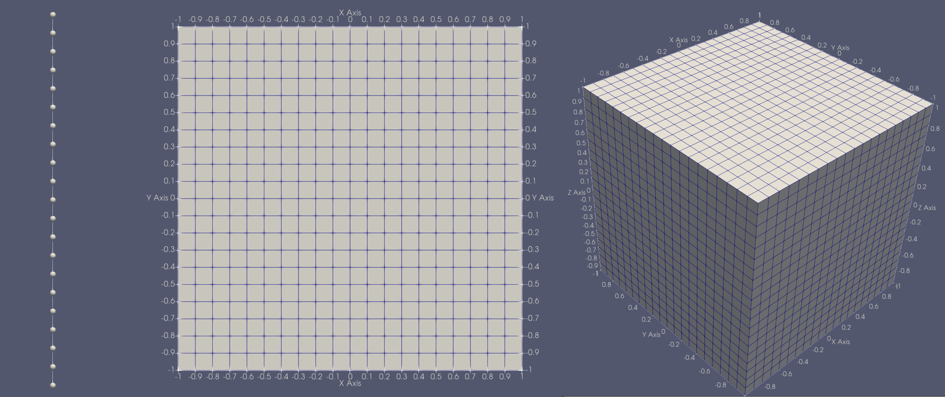
[From left to right] 1D, 2D, 3D orthogonal mesh

1.2 The Weak-form of Poisson's equation

When using the finite element method we develop the so-called weak-form by weighting the Poisson equation with a trial space function, $t_i(\mathbf{x})$ , where is a unique node in the problem, and then integrate over the volume of the domain

$-\int_V t_i \boldsymbol{\nabla} \boldsymbol{\cdot} \bigr(\boldsymbol{\nabla} \phi(\mathbf{x})\bigr) dV = \int_V t_i q(\mathbf{x}) dV.$

Next we apply integration by parts to the left term, for which,

$t_i \boldsymbol{\nabla} \boldsymbol{\cdot} \bigr(\boldsymbol{\nabla} \phi(\mathbf{x})\bigr) = \boldsymbol{\nabla} \cdot (t_i \boldsymbol{\nabla} \phi) - (\boldsymbol{\nabla} t_i ) \boldsymbol{\cdot} (\boldsymbol{\nabla} \phi)$

which gives

$\int_V (\boldsymbol{\nabla} t_i ) \boldsymbol{\cdot} (\boldsymbol{\nabla} \phi) dV -\int_V \boldsymbol{\nabla} \boldsymbol{\cdot} (t_i \boldsymbol{\nabla} \phi) dV = \int_V t_i q(\mathbf{x}) dV.$

We then apply Gauss's Divergence Theorem to the second term from the left, to get

$\int_V (\boldsymbol{\nabla} t_i ) \boldsymbol{\cdot} (\boldsymbol{\nabla} \phi) dV -\int_S \mathbf{n} \boldsymbol{\cdot} (t_i \boldsymbol{\nabla} \phi) dA = \int_V t_i q(\mathbf{x}) dV.$

This is essentially the weak-form.

1.3 The discretized equation with the Continuous Galerkin approach

To fully discretize this equation we next approximate the continuous nature of $\phi(\mathbf{x})$ using essentially a very fancy interpolation scheme. With this scheme we approximate $\phi(\mathbf{x})$ as $\phi_h(\mathbf{x})$ where

$\phi(\mathbf{x}) \approx \phi_h(\mathbf{x}) = \sum_j \phi_j b_j(\mathbf{x})$

where the coefficients $\phi_j$ do not dependent on space and $b_j(\mathbf{x})$ are called shape functions. For this tutorial we will be utilizing the Piecewise Linear Continuous (PWLC) shape functions which are generally specially in the fact that they can support arbitrary polygons and polyhedra.

We will also follow a Galerkin approach, resulting in the trial-functions being the same as the shape functions, i.e., $t_n(\mathbf{x}) = b_n(\mathbf{x})$ .

With this approximation defined, our weak form, after neglecting the surface integral since we have Dirichlet boundary conditions, becomes

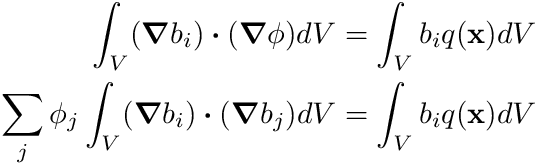
$\begin{align*} \int_V (\boldsymbol{\nabla} b_i ) \boldsymbol{\cdot} (\boldsymbol{\nabla} \phi) dV &= \int_V b_i q(\mathbf{x}) dV \\ \sum_j \phi_j \int_V (\boldsymbol{\nabla} b_i ) \boldsymbol{\cdot} (\boldsymbol{\nabla} b_j) dV &= \int_V b_i q(\mathbf{x}) dV \end{align*}$

Now we are faced with the dilemma of how to compute the integral terms in this equation. The first thing we do here is to observe that the shape functions are defined cell-by-cell, therefore we can drill a little deeper by defining

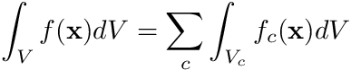
$\begin{align*} \int_V f(\mathbf{x}) dV &= \sum_c \int_{V_c} f_c(\mathbf{x}) dV \\ \end{align*}$

where is the volume of cell . The function is a function uniquely defined within cell 's volume.

These integrals are often difficult to perform in real-world coordinates and are therefore carried out on a reference element in a different coordinate system. This necessitates the use of a transformation using the magnitude of the Jacobian that transforms the above integrals into the form

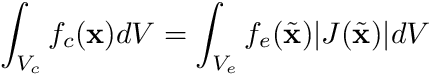
$\begin{align*} \int_{V_c} f_c(\mathbf{x}) dV &= \int_{V_e} f_e(\tilde{\mathbf{x}}) |J(\tilde{\mathbf{x}})| dV \end{align*}$

where $\tilde{\mathbf{x}}$ is position in the reference coordinate frame, $|J(\tilde{\mathbf{x}})|$ is the magnitude of the Jacobian, is the volume of the reference element, and is the reference element equivalent of . Now, the big advantage of doing this is that we can use quadrature rules for these integrals

$\begin{align*} \int_{V_e} f_e(\tilde{\mathbf{x}}) |J(\tilde{\mathbf{x}})| dV &= \sum_n w_n f_e(\tilde{\mathbf{x}}_n) |J(\tilde{\mathbf{x}}_n)| \end{align*}$

where $\tilde{\mathbf{x}}_n$ are the abscissas of the quadrature rule and are the quadrature weights.

With these mathematical formulations defined we can write

$\begin{align*} \sum_j \phi_j \sum_c \sum_n^{N_V} \biggr[ w_n (\boldsymbol{\nabla} b_i(\tilde{\mathbf{x}}_n) ) \boldsymbol{\cdot} (\boldsymbol{\nabla} b_j(\tilde{\mathbf{x}}_n)) |J(\tilde{\mathbf{x}}_n)| \biggr] &= \sum_c \sum_n^{N_V} w_n b_i(\tilde{\mathbf{x}}_n) q(\tilde{\mathbf{x}}_n \to \mathbf{x}) |J(\tilde{\mathbf{x}}_n)| \end{align*}$

2 Setting up the problem

For this tutorial we basically follow the flow of Coding Tutorial 1 - Poisson's problem with Finite Volume. Make sure you make sensible changes to the CMakeLists.txt file and name your source file appropriately, which for me is code_tut3.cc.

The first portion of the tutorial is the same. We create a mesh.lua file in the chi_build directory. We get the grid

int main(int argc, char* argv[])
{
  chi::Initialize(argc,argv);
  chi::RunBatch(argc, argv);
 
  chi::log.Log() << "Coding Tutorial 3";
 
  //============================================= Get grid
  auto grid_ptr = chi_mesh::GetCurrentHandler().GetGrid();
  const auto& grid = *grid_ptr;
 
  chi::log.Log() << "Global num cells: " << grid.GetGlobalNumberOfCells();

3 Initializing the PWLC Spatial Discretization

To gain access to the chi_math::SpatialDiscretization_PWLC class we need to include the header

#include "math/SpatialDiscretization/FiniteElement/PiecewiseLinear/pwlc.h"

Next we add the following code

//============================================= Make SDM
typedef std::shared_ptr<chi_math::SpatialDiscretization> SDMPtr;
SDMPtr sdm_ptr = chi_math::SpatialDiscretization_PWLC::New(grid_ptr);
const auto& sdm = *sdm_ptr;
 
const auto& OneDofPerNode = sdm.UNITARY_UNKNOWN_MANAGER;
 
const size_t num_local_dofs = sdm.GetNumLocalDOFs(OneDofPerNode);
const size_t num_globl_dofs = sdm.GetNumGlobalDOFs(OneDofPerNode);
 
chi::log.Log() << "Num local DOFs: " << num_local_dofs;
chi::log.Log() << "Num globl DOFs: " << num_globl_dofs;

The initialization of the matrices and vectors remain exactly the same as in the Finite Volume tutorial:

//============================================= Initializes Mats and Vecs
const auto n = static_cast<int64_t>(num_local_dofs);
const auto N = static_cast<int64_t>(num_globl_dofs);
Mat A;
Vec x,b;
 
A = chi_math::PETScUtils::CreateSquareMatrix(n,N);
x = chi_math::PETScUtils::CreateVector(n,N);
b = chi_math::PETScUtils::CreateVector(n,N);
 
std::vector<int64_t> nodal_nnz_in_diag;
std::vector<int64_t> nodal_nnz_off_diag;
sdm.BuildSparsityPattern(nodal_nnz_in_diag,nodal_nnz_off_diag, OneDofPerNode);
 
chi_math::PETScUtils::InitMatrixSparsity(A,
                                         nodal_nnz_in_diag,
                                         nodal_nnz_off_diag);

4 Using quadrature data to assemble the system

With the finite element method the conventional way to assemble the matrix is to do so by element (even though continuous FEM is only concerned about nodes). Therefore we start with a loop over elements then assemble our discretized equation

$\begin{align*} \sum_j \phi_j \sum_c \sum_n^{N_V} \biggr[ w_n (\boldsymbol{\nabla} b_i(\tilde{\mathbf{x}}_n) ) \boldsymbol{\cdot} (\boldsymbol{\nabla} b_j(\tilde{\mathbf{x}}_n)) |J(\tilde{\mathbf{x}}_n)| \biggr] &= \sum_c \sum_n^{N_V} w_n b_i(\tilde{\mathbf{x}}_n) q(\tilde{\mathbf{x}}_n \to \mathbf{x}) |J(\tilde{\mathbf{x}}_n)| \end{align*}$

For which the first portion of the code is

for (const auto& cell : grid.local_cells)
{
  const auto& cell_mapping = sdm.GetCellMapping(cell);
  const auto  qp_data      = cell_mapping.MakeVolumeQuadraturePointData();
 
  const size_t num_nodes = cell_mapping.NumNodes();
  MatDbl Acell(num_nodes, VecDbl(num_nodes, 0.0));
  VecDbl cell_rhs(num_nodes, 0.0);
 
  for (size_t i=0; i<num_nodes; ++i)
  {
    for (size_t j=0; j<num_nodes; ++j)
    {
      double entry_aij = 0.0;
      for (size_t qp : qp_data.QuadraturePointIndices())
      {
        entry_aij +=
          qp_data.ShapeGrad(i, qp).Dot(qp_data.ShapeGrad(j, qp)) *
          qp_data.JxW(qp);
      }//for qp
      Acell[i][j] = entry_aij;
    }//for j
    for (size_t qp : qp_data.QuadraturePointIndices())
      cell_rhs[i] += 1.0 * qp_data.ShapeValue(i, qp) * qp_data.JxW(qp);
  }//for i
  //
  // More code not shown
  //

The first thing we do here, as with any SD, is to grab the relevant cell mapping. After that we immediately create a chi_math::finite_element::InternalQuadraturePointData with the line of code

const auto qp_data = cell_mapping.MakeVolumeQuadraturePointData();

This data structure contains the shape function values, together with other data, pre-stored per quadrature point.

Next we create a local cell-matrix and local right-hand-side (RHS) which serve as lightweight proxies before we assemble relevant values into the global matrix and global RHS.

const size_t num_nodes = cell_mapping.NumNodes();
MatDbl Acell(num_nodes, VecDbl(num_nodes, 0.0));
VecDbl cell_rhs(num_nodes, 0.0);

We then loop over all the node combinations of our equation above but with scope only on the local element. Notice that we never actually pass around the actual quadrature points but rather use the quadrature point indices via qp_data.QuadraturePointIndices().

for (size_t i=0; i<num_nodes; ++i)
{
  for (size_t j=0; j<num_nodes; ++j)
  {
    double entry_aij = 0.0;
    for (size_t qp : qp_data.QuadraturePointIndices())
    {
      entry_aij +=
        qp_data.ShapeGrad(i, qp).Dot(qp_data.ShapeGrad(j, qp)) *
        qp_data.JxW(qp);
    }//for qp
    Acell[i][j] = entry_aij;
  }//for j
  for (size_t qp : qp_data.QuadraturePointIndices())
    cell_rhs[i] += 1.0 * qp_data.ShapeValue(i, qp) * qp_data.JxW(qp);
}//for i

Notice that we are actually doing

$\begin{align*} \sum_j \sum_n^{N_V} \biggr[ (\boldsymbol{\nabla} b_i(\tilde{\mathbf{x}}_n) ) \boldsymbol{\cdot} (\boldsymbol{\nabla} b_j(\tilde{\mathbf{x}}_n)) w_n |J(\tilde{\mathbf{x}}_n)| \biggr] \end{align*}$

for cell , where $w_n |J(\tilde{\mathbf{x}}_n)|$ is combined into qp_data.JxW(qp).

5 Compensating for Dirichlet boundaries

Dirichlet requires some special considerations. The equation for node essentially becomes $\phi_i = 0$ for our case of zero Dirichlet boundary conditions. This essentially places just a 1 on the diagonal with no entries off-diagonal for the entire row . Therefore, we need to modify the local cell-matrix to reflect this situation.

We are unfortunately not done yet. Any row in the matrix that has an off-diaganol entry that corresponds to column will need to be moved to the RHS. This is because it could destroy the symmetry of an otherwise symmetric matrix.

We handle both these modifications in the following way. We build a flag-list for each cell node

std::vector<bool> node_boundary_flag(num_nodes, false);
const size_t num_faces = cell.faces.size();
for (size_t f=0; f<num_faces; ++f)
{
  const auto& face = cell.faces[f];
  if (face.has_neighbor) continue;
 
  const size_t num_face_nodes = face.vertex_ids.size();
  for (size_t fi=0; fi<num_face_nodes; ++fi)
  {
    const uint i = cell_mapping.MapFaceNode(f,fi);
    node_boundary_flag[i] = true;
  }//for fi
}//for face f

Notice the use of face.has_neighbor here. If the face does not have a neighbor it means the face is on a boundary and therefore a Dirichlet node. Once this condition applies we loop over the face nodes, map the face-node to a cell-node then flag that node as being on a boundary.

Finally, we now assemble the local cell-matrix and local RHS into the global system.

//======================= Assembly into system
for (size_t i=0; i<num_nodes; ++i)
{
  if (node_boundary_flag[i]) //if dirichlet node
  {
    MatSetValue(A, imap[i], imap[i], 1.0, ADD_VALUES);
    VecSetValue(b, imap[i], 0.0, ADD_VALUES);
  }
  else
  {
    for (size_t j=0; j<num_nodes; ++j)
    {
      if (not node_boundary_flag[j])
        MatSetValue(A, imap[i], imap[j], Acell[i][j], ADD_VALUES);
    }//for j
    VecSetValue(b, imap[i], cell_rhs[i], ADD_VALUES);
  }
}//for i

We essentially loop over each node, after which we have two conditions: if the node is a boundary node then we just add an entry on the diagonal, if the node is not a boundary node we then loop over the row entries. We perform a check again to see if the j-entries are boundary nodes. If they are we put them on the RHS, if they are not then they are allowed to be matrix entries.

After this process we assemble the matrix and the RHS globally like we did before:

chi::log.Log() << "Global assembly";
 
MatAssemblyBegin(A, MAT_FINAL_ASSEMBLY);
MatAssemblyEnd(A, MAT_FINAL_ASSEMBLY);
VecAssemblyBegin(b);
VecAssemblyEnd(b);
 
chi::log.Log() << "Done global assembly";

6 Solving and visualizing

Solving the system and visualizing it is the same as was done for the Finite Volume tutorial. The matrix is still Symmetric Positive Definite (SPD) so we use the same solver/precondtioner setup.

//============================================= Create Krylov Solver
chi::log.Log() << "Solving: ";
auto petsc_solver =
  chi_math::PETScUtils::CreateCommonKrylovSolverSetup(
    A,               //Matrix
    "PWLCDiffSolver",  //Solver name
    KSPCG,           //Solver type
    PCGAMG,          //Preconditioner type
    1.0e-6,          //Relative residual tolerance
    1000);            //Max iterations
 
//============================================= Solve
KSPSolve(petsc_solver.ksp,b,x);
 
chi::log.Log() << "Done solving";
 
//============================================= Extract PETSc vector
std::vector<double> field;
sdm.LocalizePETScVector(x,field,OneDofPerNode);
 
//============================================= Clean up
KSPDestroy(&petsc_solver.ksp);
 
VecDestroy(&x);
VecDestroy(&b);
MatDestroy(&A);
 
chi::log.Log() << "Done cleanup";
 
//============================================= Create Field Function
auto ff = std::make_shared<chi_physics::FieldFunction>(
  "Phi",                                           //Text name
  sdm_ptr,                                         //Spatial Discr.
  chi_math::Unknown(chi_math::UnknownType::SCALAR) //Unknown
);
 
ff->UpdateFieldVector(field);
 
ff->ExportToVTK("CodeTut3_PWLC");

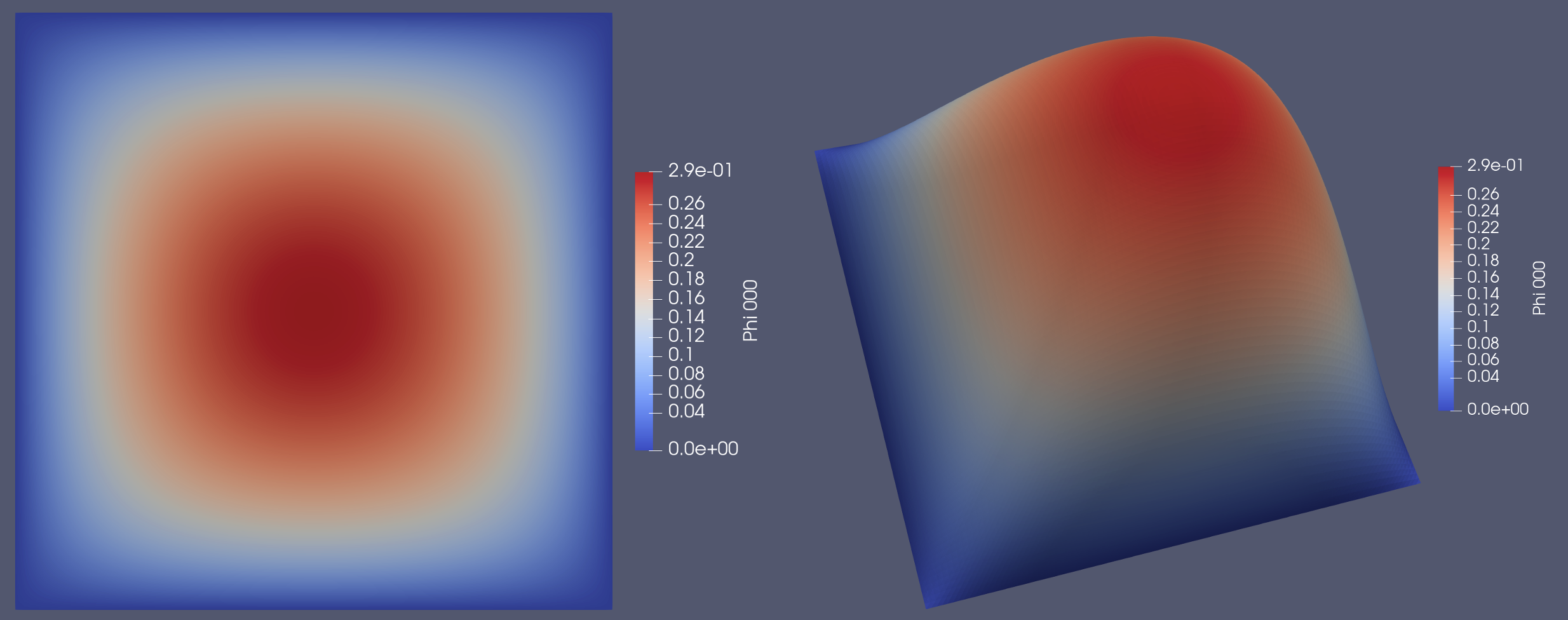
Solution for a 2D mesh with a flat and warped view

The complete program

#include "chi_runtime.h"
#include "chi_log.h"
 
#include "mesh/MeshHandler/chi_meshhandler.h"
 
#include "math/SpatialDiscretization/FiniteElement/PiecewiseLinear/pwlc.h"
#include "math/PETScUtils/petsc_utils.h"
 
#include "physics/FieldFunction/fieldfunction2.h"
 
int main(int argc, char* argv[])
{
  chi::Initialize(argc,argv);
  chi::RunBatch(argc, argv);
 
  chi::log.Log() << "Coding Tutorial 3";
 
  //============================================= Get grid
  auto grid_ptr = chi_mesh::GetCurrentHandler().GetGrid();
  const auto& grid = *grid_ptr;
 
  chi::log.Log() << "Global num cells: " << grid.GetGlobalNumberOfCells();
 
  //============================================= Make SDM
  typedef std::shared_ptr<chi_math::SpatialDiscretization> SDMPtr;
  SDMPtr sdm_ptr = chi_math::SpatialDiscretization_PWLC::New(grid_ptr);
  const auto& sdm = *sdm_ptr;
 
  const auto& OneDofPerNode = sdm.UNITARY_UNKNOWN_MANAGER;
 
  const size_t num_local_dofs = sdm.GetNumLocalDOFs(OneDofPerNode);
  const size_t num_globl_dofs = sdm.GetNumGlobalDOFs(OneDofPerNode);
 
  chi::log.Log() << "Num local DOFs: " << num_local_dofs;
  chi::log.Log() << "Num globl DOFs: " << num_globl_dofs;
 
  //============================================= Initializes Mats and Vecs
  const auto n = static_cast<int64_t>(num_local_dofs);
  const auto N = static_cast<int64_t>(num_globl_dofs);
  Mat A;
  Vec x,b;
 
  A = chi_math::PETScUtils::CreateSquareMatrix(n,N);
  x = chi_math::PETScUtils::CreateVector(n,N);
  b = chi_math::PETScUtils::CreateVector(n,N);
 
  std::vector<int64_t> nodal_nnz_in_diag;
  std::vector<int64_t> nodal_nnz_off_diag;
  sdm.BuildSparsityPattern(nodal_nnz_in_diag,nodal_nnz_off_diag, OneDofPerNode);
 
  chi_math::PETScUtils::InitMatrixSparsity(A,
                                           nodal_nnz_in_diag,
                                           nodal_nnz_off_diag);
 
  //============================================= Assemble the system
  chi::log.Log() << "Assembling system: ";
  for (const auto& cell : grid.local_cells)
  {
    const auto& cell_mapping = sdm.GetCellMapping(cell);
    const auto  qp_data      = cell_mapping.MakeVolumeQuadraturePointData();
 
    const size_t num_nodes = cell_mapping.NumNodes();
    MatDbl Acell(num_nodes, VecDbl(num_nodes, 0.0));
    VecDbl cell_rhs(num_nodes, 0.0);
 
    for (size_t i=0; i<num_nodes; ++i)
    {
      for (size_t j=0; j<num_nodes; ++j)
      {
        double entry_aij = 0.0;
        for (size_t qp : qp_data.QuadraturePointIndices())
        {
          entry_aij +=
            qp_data.ShapeGrad(i, qp).Dot(qp_data.ShapeGrad(j, qp)) *
            qp_data.JxW(qp);
        }//for qp
        Acell[i][j] = entry_aij;
      }//for j
      for (size_t qp : qp_data.QuadraturePointIndices())
        cell_rhs[i] += 1.0 * qp_data.ShapeValue(i, qp) * qp_data.JxW(qp);
    }//for i
 
    //======================= Flag nodes for being on dirichlet boundary
    std::vector<bool> node_boundary_flag(num_nodes, false);
    const size_t num_faces = cell.faces.size();
    for (size_t f=0; f<num_faces; ++f)
    {
      const auto& face = cell.faces[f];
      if (face.has_neighbor) continue;
 
      const size_t num_face_nodes = face.vertex_ids.size();
      for (size_t fi=0; fi<num_face_nodes; ++fi)
      {
        const uint i = cell_mapping.MapFaceNode(f,fi);
        node_boundary_flag[i] = true;
      }//for fi
    }//for face f
 
    //======================= Develop node mapping
    std::vector<int64_t> imap(num_nodes, 0); //node-mapping
    for (size_t i=0; i<num_nodes; ++i)
      imap[i] = sdm.MapDOF(cell, i);
 
    //======================= Assembly into system
    for (size_t i=0; i<num_nodes; ++i)
    {
      if (node_boundary_flag[i]) //if dirichlet node
      {
        MatSetValue(A, imap[i], imap[i], 1.0, ADD_VALUES);
        VecSetValue(b, imap[i], 0.0, ADD_VALUES);
      }
      else
      {
        for (size_t j=0; j<num_nodes; ++j)
        {
          if (not node_boundary_flag[j])
            MatSetValue(A, imap[i], imap[j], Acell[i][j], ADD_VALUES);
        }//for j
        VecSetValue(b, imap[i], cell_rhs[i], ADD_VALUES);
      }
    }//for i
  }//for cell
 
  chi::log.Log() << "Global assembly";
 
  MatAssemblyBegin(A, MAT_FINAL_ASSEMBLY);
  MatAssemblyEnd(A, MAT_FINAL_ASSEMBLY);
  VecAssemblyBegin(b);
  VecAssemblyEnd(b);
 
  chi::log.Log() << "Done global assembly";
 
  //============================================= Create Krylov Solver
  chi::log.Log() << "Solving: ";
  auto petsc_solver =
    chi_math::PETScUtils::CreateCommonKrylovSolverSetup(
      A,               //Matrix
      "PWLCDiffSolver",  //Solver name
      KSPCG,           //Solver type
      PCGAMG,          //Preconditioner type
      1.0e-6,          //Relative residual tolerance
      1000);            //Max iterations
 
  //============================================= Solve
  KSPSolve(petsc_solver.ksp,b,x);
 
  chi::log.Log() << "Done solving";
 
  //============================================= Extract PETSc vector
  std::vector<double> field;
  sdm.LocalizePETScVector(x,field,OneDofPerNode);
 
  //============================================= Clean up
  KSPDestroy(&petsc_solver.ksp);
 
  VecDestroy(&x);
  VecDestroy(&b);
  MatDestroy(&A);
 
  chi::log.Log() << "Done cleanup";
 
  //============================================= Create Field Function
  auto ff = std::make_shared<chi_physics::FieldFunction>(
    "Phi",                                           //Text name
    sdm_ptr,                                         //Spatial Discr.
    chi_math::Unknown(chi_math::UnknownType::SCALAR) //Unknown
  );
 
  ff->UpdateFieldVector(field);
 
  ff->ExportToVTK("CodeTut3_PWLC");
 
  chi::Finalize();
  return 0;
}

Table of contents