The chi_math::UnknownManager

Table of contents

• Introduction
• 1 Cells vs Vertices vs Nodes vs Degree-of-Freedom (DOF)
• 2 One DOF per node
• 3 Multiple DOFs Nodal ordering
• 4 Multiple DOFs Block ordering

Introduction

As a developer you might come across code such as

imap[i] = sdm.MapDOF(cell, i);

or its more elaborate cousin

const int64_t imap = m_sdm.MapDOF(cell,i,m_uk_man,0,g);

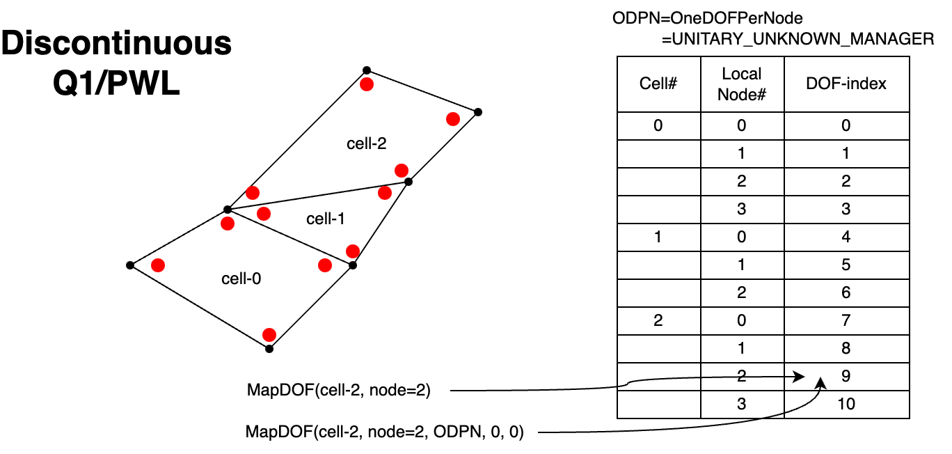
The two function calls, MapDOF with 2 arguments and MapDOF with 5 arguments, are both methods of the base-class chi_math::SpatialDiscretization.

The two overloaded methods, chi_math::SpatialDiscretization::MapDOF return the global index of a degree-of-freedom (DOF). The counterparts to MapDOF are the MapDOFLocal methods that provide the local index of a DOF.

These functions are called with either 2 arguments

• A cell reference
• A cell-node local-index

or with 5 arguments

• A cell reference
• A cell-node local-index
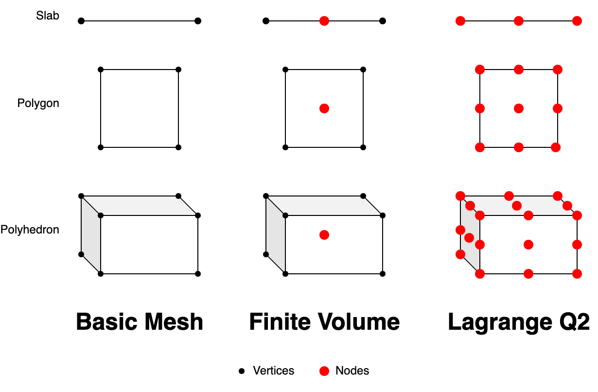
• An unknown-manager (chi_math::UnknownManager)
• An unknown id
• A component id

1 Cells vs Vertices vs Nodes vs Degree-of-Freedom (DOF)

These comparisons are conceptually simple. The geometry of a cell is described by its vertices (see Figure 1 below). The mesh cannot be completely defined without the vertices, therefore, cells always go hand-in-hand with vertices.

A spatial discretization (e.g., Finite Volume, PWL, Lagrange Q1, Lagrange Q2) places nodes on the mesh that may or may not coincide with some of the vertices. For example, the Finite Volume spatial discretization places a single node for each cell, at the cell's centroid (hence no coincidence with any vertex), whilst a Lagrange Q2 spatial discretization has some of its nodes on the vertices while other are not (see Figure 1 below).

Figure 1: Cells, vertices and nodes.

Where degrees-of-freedom differ from nodes is that each node can be stacked with a number of unknowns, e.g., one might have to solve a number of physical variables in a multiphysics simulation involving 2D velocity, and , a three energy group flux, , and pressure, . One can stack these variables in any form, for example:

• Unknown 0, a 6 component vector containing , and

or more elegantly

• Unknown 0, a 2 component vector containing and
• Unknown 1, a 3 component vector containing
• Unknown 2, a single scalar (1 component) containing just

The latter essentially means that each node can have a number of unknowns stacked onto it as shown in Figure 2 below.

Figure 2: Unknowns/DOFs stacked onto a node

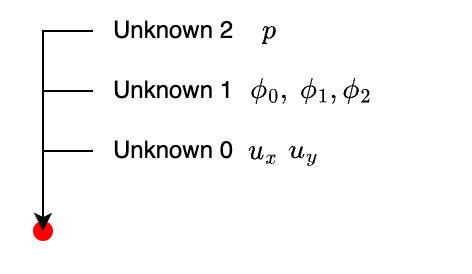
The individual components of the unknowns are unique for every node and are called the degrees-of-freedom (DOFs).

2 One DOF per node

All the spatial discretizations have a default unknown-manager, defined during initialization, called UNITARY_UNKNOWN_MANAGER. This allows the spatial discretization to map indices as shown in Figure 3 below

Figure 3: Mapping One DOF per Node

3 Multiple DOFs Nodal ordering

With multiple unknowns like the 2D velocity, multigroup flux, and pressure example above we can create an unknown manager with this structure as follows

chi_math::UnknownManager uk_man;
uk_man.AddUnknown(chi_math::UnknownType::VECTOR_2);    //u_x, u_y
uk_man.AddUnknown(chi_math::UnknownType::VECTOR_N, 3); //phi_0 to phi_2
uk_man.AddUnknown(chi_math::UnknownType::SCALAR);      //pressure

Using this unknown manager to map DOFs is then done as shown below in Figure 4.

Figure 4: Mapping with a nodal ordering

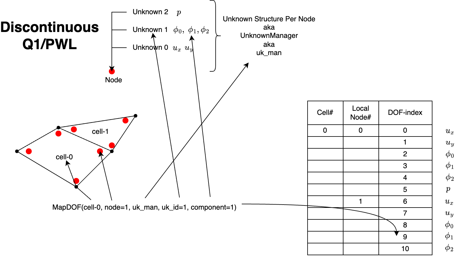
Notice here that the ordering is per-node, i.e., for each node the DOFs all the DOFs are stacked into a vector before moving to a new node. This is the default ordering in ChiTech.

4 Multiple DOFs Block ordering

To create a Block-ordered vector mapping the only modification needed is in the constructor of the unknown manager:

chi_math::UnknownManager uk_man(chi_math::UnknownStorageType::BLOCK);
uk_man.AddUnknown(chi_math::UnknownType::VECTOR_2);    //u_x, u_y
uk_man.AddUnknown(chi_math::UnknownType::VECTOR_N, 3); //phi_0 to phi_2
uk_man.AddUnknown(chi_math::UnknownType::SCALAR);      //pressure

Now that we specified that we should use chi_math::UnknownStorageType::BLOCK the unknown manager maps as shown in Figure 5 below

Figure 5: Mapping with a block ordering

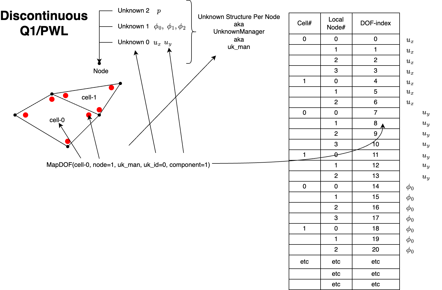
Block ordering is likely desireable if one wishes to apply block-solves.