1 Introduction

Monte Carlo based flux estimators traditionally use a number of tracks, traced within a volume, to estimate the scalar flux. For amount of tracks traced inside a volume, , originating from a sample of number of particles/rays, the scalar flux, $\phi$ , can be estimated with

$\phi \approx \frac{1}{N_p V} \sum_t^{N_t} \ell_t,$

where $\ell_t$ is the -th track length. This simply means that the scalar flux is the "average track length per unit volume".

The individual tracks of these particles can be assigned a weight, , enabling a multitude of features.

$\phi \approx \frac{1}{N_p V} \sum_t^{N_t} \ell_t w_t,$

For our purposes we are interested in three possible weightings, i) weighting by a spherical harmonic, which can be used to compute flux moments, ii) weighting by average FE shape function values, allowing the projection of flux onto a FE space, and finally iii) weighting with an exponential attenuation, allowing the computation of uncollided flux.

1.1 Weighting with a spherical harmonic

Applying a weight with a spherical harmonic is conceptually simple. For the -th track we simply set the weight to the spherical harmonic evaluated with the direction, $\boldsymbol{\Omega}_t$ , of the track,

$\phi_{\ell m} \approx \frac{1}{N_p V} \sum_t^{N_t} \ell_t Y_{\ell m}( \boldsymbol{\Omega}_t),$

1.2 Weighting by average FE shape function values

For a DFEM projection of the fluxes we require nodal values, on each cell, for a given flux quantity, $\phi$ . Therefore we seek $\phi_h$ such that

$\begin{eqnarray*} \int_V b_i \phi_h dV = \int_V b_i \phi dV \end{eqnarray*}$

and since $\phi_h = \sum_j b_j \phi_j$ we need to solve the cell-by-cell system defined by

$\begin{eqnarray*} \sum_j \phi_j \int_V b_i b_j dV = \int_V b_i \phi dV. \end{eqnarray*}$

In this system the entries 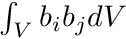$\int_V b_i b_j dV$ are simply the entries of the mass matrix, 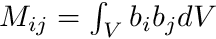$M_{ij} = \int_V b_i b_j dV$ , and we still need to find the rhs-entries 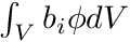$\int_V b_i \phi dV$ . This is where we will use the track length based estimators by weighting with the shape functions b_i.

In this formulation we have

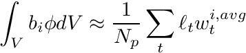
$\begin{eqnarray*} \int_V b_i \phi dV \approx \frac{1}{N_p} \sum_t \ell_t w_t^{i,avg} \end{eqnarray*}$

where

$w_t^{i,avg} = \frac{ \int_{s_a}^{s_b} b_i(s\mapsto \mathbf{x}) ds } {\int_{s_a}^{s_b} ds} = \frac{ \int_{s_a}^{s_b} b_i(s\mapsto \mathbf{x}) ds } {\ell_t},$

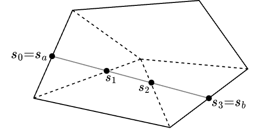
the average basis function value along the track. For ordinary Lagrange FE shape functions, which are not defined piecewise, the integral in the numerator can be obtained exactly using a numerical quadrature. For our applications, where we use the PWLD FE shape functions we need to split this integral per segment of the basic cell crossed.

For example, consider the polygon below, where a ray is traced from position to .

The track traced across the cell needs to be split into the segments defined by the sub-triangles of the polygon it crossed (for polyhedrons this would be the sub-tetrahedrons). Therefore the track $s_a \to s_b$ needs to be split into tracks $s_0 \to s_1$ , $s_1 \to s_2$ and $s_2 \to s_3$ as per the figure. Therefore the integral becomes

$\int_{s_a}^{s_b} b_i(s\mapsto \mathbf{x}) ds = \int_{s_0}^{s_1} b_i(s\mapsto \mathbf{x}) ds + \int_{s_1}^{s_2} b_i(s\mapsto \mathbf{x}) ds + \int_{s_2}^{s_3} b_i(s\mapsto \mathbf{x}) ds$

which we can evaluate analytically since it is linear on each segment.

Note: The mapping of $s\mapsto \mathbf{x}$ can be quite expensive so in this particular case it would be better to evaluate the shape function at the half-way point of each segment, after which the integral becomes

$\int_{s_a}^{s_b} b_i(s\mapsto \mathbf{x}) ds = b_i(\frac{s_0 + s_1}{2}\mapsto \mathbf{x}) (s_1 - s_0) + b_i(\frac{s_1 + s_2}{2}\mapsto \mathbf{x}) (s_2 - s_1) + b_i(\frac{s_2 + s_3}{2}\mapsto \mathbf{x}) (s_3 - s_2) +$

1.3 Weighting with an exponential attenuation

Weighting with an exponential attenuation adds the final piece of weighting necessary to efficiently compute the uncollided flux.

The exponential attenuation of the uncollided flux, $\psi$ , along the path of a ray with direction $\boldsymbol{\Omega}$ is expressed as

$\frac{d\psi}{ds} = -\sigma_t(s) \psi(s)$

where is the distance traveled and $\sigma_t$ is the total cross section. From this model we can compute the attenuation across a cell, with constant $\sigma_t$ , as

$\psi(s) = \psi(s=0) e^{-\sigma_t s}$

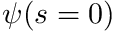where $\psi(s=0)$ is the value of $\psi$ when it entered the cell.

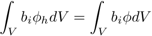
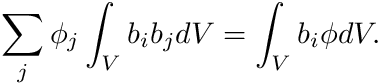
To assimilate all of this into a raytracing algorithm we start a source particle with a weight, , which acts as the proxy for $\psi$ (i.e., $w^p \equiv \psi$ ). From this we can determine the nodal uncollided flux, $\phi^{uc}$ , in a similar fashion as we would determine the regular flux, i.e.,

$\sum_j \phi_j^{uc} \int_V b_i b_j dV = \int_V b_i \phi^{uc} dV,$

however, now we need additional treatment for the integral containing $\phi^{uc}$ , for which we have

$\int_V b_i \phi^{uc} dV \approx \frac{1}{N_p} \sum_t \ell_t w_t^{i,avg},$

where, this time,

$w_t^{i,avg} = \frac{ \int_{s_a}^{s_b} w^p(s) b_i(s\mapsto \mathbf{x}) ds } {\ell_t}.$

Note here that is a function of position, specifically

$w^p(s) = w^p(s=s_a) e^{-\sigma_t s}$

and so is the basis function .

The form of this integral needs to split into segments in the same way we did in the previous subsection. Therefore, given K amount of segments, we now have

$\ell_t w_t^{i,avg} = \sum_{k=0}^{K-1} \ell_{tk} w_{tk}^{i,avg}$

where $\ell_{tk}$ is the track length of the -th segment and $w_{tk}^{i,avg}$ is the average weight of this segment. The weight is computed with

$w_{tk}^{i,avg} = \frac{ \int_{s_k}^{s_{k+1}} w^p(s) b_i(s\mapsto \mathbf{x}) ds } {\ell_{tk}}.$

where and $s_{k+1}$ are the beginning and ending positions of segment respectively.

Note here that, since we have an expression for , we can compute at any point along track including at the start of any segment. Therefore we define 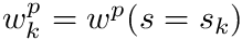which allows us to express as

$w^p(s) = w_k^p e^{-\sigma_t(s-s_k)}, \quad \quad \quad s\in[s_k,s_{k+1}]$

Additionally we express the basis functions on a segment, since we know the shape function is linear on the segment, as

$b_i(s) = b_{i,k} \frac{s_{k+1}-s}{s_{k+1}-s_k} + b_{i,k+1} \frac{s-s_k}{s_{k+1}-s_k}$

where $b_{i,k}$ and $b_{i,k+1}$ are the basis function values at the beginning and end of the segment, respectively. These two expressions allow us to evaluate the segment average weight as

$w_{tk}^{i,avg} = \frac{1}{\ell_{tk}} \int_{s_k}^{s_{k+1}} w_k^p e^{-\sigma_t(s-s_k)} \biggr[ b_{i,k} \frac{s_{k+1}-s}{s_{k+1}-s_k} + b_{i,k+1} \frac{s-s_k}{s_{k+1}-s_k} \biggr] ds$

and since 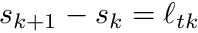$s_{k+1}-s_k = \ell_{tk}$ we can simplify this expression as

$\begin{align*} w_{tk}^{i,avg} &= \frac{1}{\ell_{tk}} \int_{0}^{\ell_{tk}} w_k^p e^{-\sigma_t s' } \biggr[ b_{i,k} \frac{\ell_{tk}-s'}{\ell_{tk}} + b_{i,k+1} \frac{s'}{\ell_{tk}} \biggr] ds' \\ &= \frac{1}{\ell_{tk}^2} \int_{0}^{\ell_{tk}} w_k^p e^{-\sigma_t s' } \biggr[ b_{i,k} \ell_{tk} + (b_{i,k+1} - b_{i,k} ) s' \biggr] ds' \end{align*}$

which is in the general form

$w_{tk}^{i,avg} = \frac{w_k^p}{\ell_{tk}^2} \int_{0}^{\ell_{tk}} e^{-\sigma_t s'} \biggr[ C_0 + C_1 s' \biggr] ds'$

where

$C_0 = b_{i,k} \ell_{tk}$

$C_1 = b_{i,k+1} - b_{i,k}.$

With these constants defined the expression can be evaluated analytically

$w_{tk}^{i,avg} = \frac{w_k^p}{\ell_{tk}^2} \biggr[ \frac{C_0}{\sigma_t} (1-e^{-\sigma_t \ell_{tk}}) + \frac{C_1}{\sigma_t^2} \biggr( 1 - (1 + \sigma_t \ell_{tk} ) \biggr)e^{-\sigma_t \ell_{tk}} \biggr]$

2 Program setup

We start by getting the grid as usual:

auto grid_ptr = chi_mesh::GetCurrentHandler().GetGrid();
const auto& grid = *grid_ptr;
 
chi::log.Log() << "Global num cells: " << grid.GetGlobalNumberOfCells();
 
const int dimension = (grid.Attributes() & chi_mesh::DIMENSION_1)? 1 :
                      (grid.Attributes() & chi_mesh::DIMENSION_2)? 2 :
                      (grid.Attributes() & chi_mesh::DIMENSION_3)? 3 : 0;

Note here that we grab the dimension.

Next we set a number of parameters important to the simulation:

const size_t num_groups = 1;
const size_t scattering_order = 1;
const auto& L = scattering_order;
const size_t num_moments =
  (dimension == 1)? L + 1 :
  (dimension == 2)? (L+1)*(L+2)/2 :
  (dimension == 3)? (L+1)*(L+1) : 0;
const double sigma_t = 0.27;
 
// Build harmonic map
std::vector<std::pair<int,int>> m_to_ell_em_map;
if (dimension == 1)
  for (int ell=0; ell<=scattering_order; ell++)
    m_to_ell_em_map.emplace_back(ell,0);
else if (dimension == 2)
  for (int ell=0; ell<=scattering_order; ell++)
    for (int m=-ell; m<=ell; m+=2)
      m_to_ell_em_map.emplace_back(ell,m);
else if (dimension == 3)
  for (int ell=0; ell<=scattering_order; ell++)
    for (int m=-ell; m<=ell; m++)
      m_to_ell_em_map.emplace_back(ell,m);

The interesting items here includes the scattering_order and the map from linear moment index to harmonic indices, m_to_ell_em_map. See the LBS Whitepaper for the detail of this but in a nutshell... Only some of the harmonics are relevant in certain dimensions.

Next we build the spatial discretization, which in this case would be a PWLD discretization, and we do this as normal:

typedef std::shared_ptr<chi_math::SpatialDiscretization> SDMPtr;
SDMPtr sdm_ptr = chi_math::SpatialDiscretization_PWLD::New(grid_ptr);
const auto& sdm = *sdm_ptr;

For the unknown manager and DOF-counts we build an unknown manager as follows:

chi_math::UnknownManager phi_uk_man;
for (size_t m=0; m<num_moments; ++m)
  phi_uk_man.AddUnknown(chi_math::UnknownType::VECTOR_N, num_groups);

And then grab the dof-counts

const size_t num_fem_local_dofs = sdm.GetNumLocalDOFs(phi_uk_man);
const size_t num_fem_globl_dofs = sdm.GetNumGlobalDOFs(phi_uk_man);
 
chi::log.Log() << "Num local FEM DOFs: " << num_fem_local_dofs;
chi::log.Log() << "Num globl FEM DOFs: " << num_fem_globl_dofs;

This allows us to define the business end, which is the flux tally vector:

std::vector<double> phi_tally(num_fem_local_dofs, 0.0);

3 The particle/ray data structure

The particle/ray data structure is the packet of data that we will be sending around in our ray tracing algorithm. First we need the basic structure:

typedef chi_mesh::Vector3 Vec3;
struct Particle
{
  Vec3 position = {0.0,0.0,0.0};
  Vec3 direction = {0.0,0.0,0.0};
  int  energy_group = 0;
  double weight = 1.0;
 
  uint64_t cell_id = 0;
 
  bool alive = true;
};

This is all basic stuff. Essentially the particle's state is tracked with the members position, direction, energy_group and weight. The other two members are simply auxiliary items to assist with the transport process.

Next we define a source, along with the determining which cell contains the source:

const Vec3 source_pos = {0.0,0.0,0.0};
 
chi_mesh::Cell const* source_cell_ptr = nullptr;
 
for (auto& cell : grid.local_cells)
  if (grid.CheckPointInsideCell(cell, source_pos))
  {
    source_cell_ptr = &cell;
    break;
  }
if (source_cell_ptr == nullptr)
  throw std::logic_error(fname + ": Source cell not found.");
 
const uint64_t source_cell_id = source_cell_ptr->global_id;

Notice here we used the grid utility CheckPointInsideCell.

4 Utility lambdas

In this section we define 3 utility functions in the form of c++ lambdas. i) A routine to sample a random direction. This gets used when we sample the source. ii) A routine to contribute a track to a PWLD tally. This is very complicated and will be explained. iii) A routine to approximate a given cell's size. The approximate cell sizes are used by the raytracer (which we will discuss later) to set appropriate tolerances used during the sub-routines of the raytracer.

4.1 Sampling a random direction

Given a random number generator we can use two random numbers to sample the azimuthal- and polar directions. The azimuthal angle is sampled uniformly, i.e., $\varphi \in [0,2\pi]$ whilst the polar angle is determined by sampling the cosine of the polar angle uniformly, i.e., $\cos \theta = \mu \in [-1,1]$ .

chi_math::RandomNumberGenerator rng;
auto SampleRandomDirection = [&rng]()
{
  double costheta = 2.0*rng.Rand() - 1.0;
  double theta    = acos(costheta);
  double varphi   = rng.Rand()*2.0*M_PI;
 
  return chi_mesh::Vector3{sin(theta) * cos(varphi),
                           sin(theta) * sin(varphi),
                           cos(theta)};
};

It is important to note that one should only use a single random number, which, gets reused, and not define new ones since the random seed for new generators will be the same.

4.2 PWLD Tally contribution

The tally contribution routine takes a track, defined by a starting and ending position, and contributes it to the specified cell's tally information. Of course additional information about the particle creating the track is also provided, i.e., the direction, energy group index and weight at the starting position.

auto ContributePWLDTally = [&sdm,&grid,&phi_tally,&phi_uk_man,&sigma_t,
                              &num_moments,&m_to_ell_em_map](
  const chi_mesh::Cell& cell,
  const Vec3& positionA,
  const Vec3& positionB,
  const Vec3& omega,
  const int g,
  double weight)
{
  const auto& cell_mapping = sdm.GetCellMapping(cell);
  const size_t num_nodes = cell_mapping.NumNodes();
 
  const auto phi_theta = chi_math::OmegaToPhiThetaSafe(omega);
  const double phi = phi_theta.first;
  const double theta = phi_theta.second;
 
  std::vector<double> segment_lengths;
  chi_mesh::PopulateRaySegmentLengths(grid,             //input
                                      cell,             //input
                                      positionA,        //input
                                      positionB,        //input
                                      omega,            //input
                                      segment_lengths); //output
 
  std::vector<double> shape_values_k;   //At s_k
  std::vector<double> shape_values_kp1; //At s_{k+1}
 
  cell_mapping.ShapeValues(positionA,       //input
                           shape_values_k); //output
 
  double d_run_sum = 0.0;
  for (const auto& segment_length_k : segment_lengths)
  {
    d_run_sum += segment_length_k;
    const double& d = d_run_sum;
 
    cell_mapping.ShapeValues(positionA+omega*d, shape_values_kp1);
 
    const auto&   b_ik   = shape_values_k;
    const auto&   b_ikp1 = shape_values_kp1;
    const double& ell_k  = segment_length_k;
 
    for (size_t i=0; i<num_nodes; ++i)
    {
      const double C0 = b_ik[i] * ell_k;
      const double C1 = b_ikp1[i] - b_ik[i];
 
      for (size_t m=0; m < num_moments; ++m)
      {
        const int64_t dof_map = sdm.MapDOFLocal(cell, i, phi_uk_man, m, g);
 
        //================= Apply harmonic weight
        const auto& ell_em = m_to_ell_em_map.at(m);
        const int ell = ell_em.first;
        const int em = ell_em.second;
 
        double w_harmonic = chi_math::Ylm(ell, em, phi, theta);
 
        //================= Apply exponential attenuation weight
        double w_exp  = (C0 / sigma_t) * (1.0 - exp(-sigma_t * ell_k)) +
                        (C1 / (sigma_t * sigma_t)) *
                        (1.0 - (1 + sigma_t * ell_k) * exp(-sigma_t * ell_k));
               w_exp *= weight / (ell_k * ell_k);
 
        //================= Combine
        double w_avg = w_harmonic * w_exp;
 
        phi_tally[dof_map] += ell_k * w_avg ;
      }//for moment m
    }//for node i
 
    shape_values_k = shape_values_kp1;
    weight *= exp(-sigma_t * segment_length_k);
  }//for d
};

The first portion of this routine is just housekeeping,

const auto& cell_mapping = sdm.GetCellMapping(cell);
const size_t num_nodes = cell_mapping.NumNodes();
 
const auto phi_theta = chi_math::OmegaToPhiThetaSafe(omega);
const double phi = phi_theta.first;
const double theta = phi_theta.second;

We get the cell mapping, number of nodes, and we convert the direction vector to a $(\varphi, \theta)$ pair. The latter will be used for the harmonic weighting.

Next we determing the segments crossed by this track. This information is populated into a vector of segment lengths, sorted according to the direction traveled by the ray, by using the routine chi_mesh::PopulateRaySegmentLengths().

std::vector<double> segment_lengths;
chi_mesh::PopulateRaySegmentLengths(grid,             //input
                                    cell,             //input
                                    positionA,        //input
                                    positionB,        //input
                                    omega,            //input
                                    segment_lengths); //output

We then declare two vectors that will hold the shape function values at different places on the segments. We can immediately determine the shape values at since this will be at position A.

std::vector<double> shape_values_k;   //At s_k
std::vector<double> shape_values_kp1; //At s_{k+1}
 
cell_mapping.ShapeValues(positionA,       //input
                         shape_values_k); //output

Next we start looping over the segments.

double d_run_sum = 0.0;
for (const auto& segment_length_k : segment_lengths)
{
  d_run_sum += segment_length_k;
  const double& d = d_run_sum;
 
  cell_mapping.ShapeValues(positionA+omega*d, shape_values_kp1);
 
  const auto&   b_ik   = shape_values_k;
  const auto&   b_ikp1 = shape_values_kp1;
  const double& ell_k  = segment_length_k;

We determine the end position of the segment using a running sum of the total segments traversed. We then populate the shape function values at $s_{k+1}$ and rename both sets of shape function values and the segment length for convenience.

Next we loop over the nodes and moments.

for (size_t i=0; i<num_nodes; ++i)
{
  const double C0 = b_ik[i] * ell_k;
  const double C1 = b_ikp1[i] - b_ik[i];
 
  for (size_t m=0; m < num_moments; ++m)
  {
    const int64_t dof_map = sdm.MapDOFLocal(cell, i, phi_uk_man, m, g);

Once a node is identified we compute the constants C0 and C1. Also once in the moment loop we can obtain the DOF local index of the tally.

Next we compute the harmonic weighting:

const auto& ell_em = m_to_ell_em_map.at(m);
const int ell = ell_em.first;
const int em = ell_em.second;
 
double w_harmonic = chi_math::Ylm(ell, em, phi, theta);

Then we compute the exponential weighting based on the formula

$w_{tk}^{i,avg} = \frac{w_k^p}{\ell_{tk}^2} \biggr[ \frac{C_0}{\sigma_t} (1-e^{-\sigma_t \ell_{tk}}) + \frac{C_1}{\sigma_t^2} \biggr( 1 - (1 + \sigma_t \ell_{tk} ) \biggr)e^{-\sigma_t \ell_{tk}} \biggr]$

with the code

double w_exp  = (C0 / sigma_t) * (1.0 - exp(-sigma_t * ell_k)) +
                (C1 / (sigma_t * sigma_t)) *
                (1.0 - (1 + sigma_t * ell_k) * exp(-sigma_t * ell_k));
       w_exp *= weight / (ell_k * ell_k);

Finally, the average weight is computed and the tally contribution is made

double w_avg = w_harmonic * w_exp;
 
phi_tally[dof_map] += ell_k * w_avg ;

At the end of each segment being processed we copy the shape function values at $s_{k+1}$ to , preventing us from having to compute the values at again (which can be expensive). We also apply the exponential attenuation to the particle weight over the segment.

shape_values_k = shape_values_kp1;

weight *= exp(-sigma_t * segment_length_k);

4.3 Approximating cell size

To obtain a very rough estimate of a cell's size we simply determine its bounding box:

auto GetCellApproximateSize = [&grid](const chi_mesh::Cell& cell)
{
  const auto& v0 = grid.vertices[cell.vertex_ids[0]];
  double xmin = v0.x, xmax = v0.x;
  double ymin = v0.y, ymax = v0.y;
  double zmin = v0.z, zmax = v0.z;
 
  for (uint64_t vid : cell.vertex_ids)
  {
    const auto& v = grid.vertices[vid];
 
    xmin = std::min(xmin, v.x); xmax = std::max(xmax, v.x);
    ymin = std::min(ymin, v.y); ymax = std::max(ymax, v.y);
    zmin = std::min(zmin, v.z); zmax = std::max(zmax, v.z);
  }
 
  return (chi_mesh::Vector3(xmin, ymin, zmin) -
          chi_mesh::Vector3(xmax, ymax, zmax)).Norm();
};

The code here should be self explanatory.

5 The raytracer

Instantiating a chi_mesh::RayTracer object is very simple. It just needs the grid and the approximate cell sizes.

std::vector<double> cell_sizes(grid.local_cells.size(), 0.0);
for (const auto& cell : grid.local_cells)
  cell_sizes[cell.local_id] = GetCellApproximateSize(cell);
 
chi_mesh::RayTracer ray_tracer(grid, cell_sizes);

6 Executing the algorithms

The basic process of simulating all the rays is fairly simple

const size_t num_particles = 10'000'000;
for (size_t n=0; n<num_particles; ++n)
{
  if (n % size_t(num_particles/10.0) == 0)
    std::cout << "#particles = " << n << "\n";
  //====================================== Create the particle
  const auto omega = SampleRandomDirection();
  Particle particle{source_pos,     //position
                    omega,          //direction
                    0,              //e_group
                    1.0,            //weight
                    source_cell_id, //cell_id
                    true};          //alive
 
  while (particle.alive)
  {
    //=============================== Get the current cell
    const auto& cell = grid.cells[particle.cell_id];
 
    //=============================== Perform the trace
    //                                to the next surface
    auto destination_info = ray_tracer.TraceRay(cell,
                                                particle.position,
                                                particle.direction);
 
    const Vec3& end_of_track_position = destination_info.pos_f;
 
    //=============================== Make tally contribution
    const int g = particle.energy_group;
    if (sdm.type == PWLD)
      ContributePWLDTally(cell,
                          particle.position,     //positionA
                          end_of_track_position, //positionB
                          particle.direction,    //omega
                          g,                     //
                          particle.weight);      //weight at A
 
    //=============================== Process cell transfer
    //                                or death
    if (not destination_info.particle_lost)
    {
      const auto& f = destination_info.destination_face_index;
      const auto& current_cell_face = cell.faces[f];
 
      if (current_cell_face.has_neighbor)
        particle.cell_id = current_cell_face.neighbor_id;
      else
        particle.alive = false; //Death at the boundary
    }
    else
    {
      std::cout << "particle" << n << " lost "
                << particle.position.PrintStr() << " "
                << particle.direction.PrintStr() << " "
                << "\n";
      break;
    }
 
    const auto& pA = particle.position;
    const auto& pB = end_of_track_position;
    particle.weight *= exp(-sigma_t*(pB-pA).Norm()); //Attenuation
    particle.position = end_of_track_position;
  }//while ray alive
 
}//for ray n

We start the process with the loop

const size_t num_particles = 10'000'000;
for (size_t n=0; n<num_particles; ++n)
{
  if (n % size_t(num_particles/10.0) == 0)
    std::cout << "#particles = " << n << "\n";

The information printing line simply prints at each 10% of completion.

We then create a source particle/ray

const auto omega = SampleRandomDirection();
Particle particle{source_pos,     //position
                  omega,          //direction
                  0,              //e_group
                  1.0,            //weight
                  source_cell_id, //cell_id
                  true};          //alive

Next we keep transporting the particle as long as it is alive. The beginning of this loop is

while (particle.alive)
{
  //=============================== Get the current cell
  const auto& cell = grid.cells[particle.cell_id];
 
  //=============================== Perform the trace
  //                                to the next surface
  auto destination_info = ray_tracer.TraceRay(cell,
                                              particle.position,
                                              particle.direction);
 
  const Vec3& end_of_track_position = destination_info.pos_f;

After a trace we have one single track within a cell.

We then contribute the PWLD tally

ContributePWLDTally(cell,
                    particle.position,     //positionA
                    end_of_track_position, //positionB
                    particle.direction,    //omega
                    particle.energy_group, //g
                    particle.weight);      //weight at A

Next we process the transfer of the particle to the next cell. If the particle hit a cell face without a neighbor then the particle is killed (i.e., alive set to false. Under some circumstances the raytracer could also fail, resulting in a lost particle, for which we print a verbose message.

if (not destination_info.particle_lost)
{
  const auto& f = destination_info.destination_face_index;
  const auto& current_cell_face = cell.faces[f];
 
  if (current_cell_face.has_neighbor)
    particle.cell_id = current_cell_face.neighbor_id;
  else
    particle.alive = false; //Death at the boundary
}
else
{
  std::cout << "particle" << n << " lost "
            << particle.position.PrintStr() << " "
            << particle.direction.PrintStr() << " "
            << "\n";
  break;
}

Lastly we update the particle's attenuation and position

const auto& pA = particle.position;
const auto& pB = end_of_track_position;
particle.weight *= exp(-sigma_t*(pB-pA).Norm()); //Attenuation
particle.position = end_of_track_position;

7 Post-processing the tallies

The tallies up to this point are still in raw format. We need to convert them to the project fashion we want.

for (const auto& cell : grid.local_cells)
{
  //====================================== Compute mass matrix
  //                                       and its inverse
  const auto& cell_mapping = sdm.GetCellMapping(cell);
  const auto& qp_data = cell_mapping.MakeVolumeQuadraturePointData();
  const size_t num_nodes = cell_mapping.NumNodes();
 
  MatDbl M(num_nodes, VecDbl(num_nodes, 0.0));
  for (auto qp : qp_data.QuadraturePointIndices())
    for (size_t i=0; i<num_nodes; ++i)
      for (size_t j=0; j<num_nodes; ++j)
        M[i][j] += qp_data.ShapeValue(i,qp) * qp_data.ShapeValue(j, qp) *
                   qp_data.JxW(qp);
 
  auto M_inv = chi_math::Inverse(M);
 
  //====================================== Apply projection
  VecDbl b(num_nodes, 0.0);
  for (size_t m=0; m<num_moments; ++m)
    for (size_t g=0; g<num_groups; ++g)
    {
      for (size_t i=0; i<num_nodes; ++i)
      {
        const int64_t imap = sdm.MapDOFLocal(cell, i, phi_uk_man, m, g);
        b[i] = phi_tally[imap] / num_particles;
      }
 
      auto c = chi_math::MatMul(M_inv, b);
 
      for (size_t i=0; i<num_nodes; ++i)
      {
        const int64_t imap = sdm.MapDOFLocal(cell, i, phi_uk_man, m, g);
        phi_tally[imap] = c[i];
      }
    }//for group g
 
}//for cell

The first portion of the loop is simply housekeeping again

for (const auto& cell : grid.local_cells)
{
  //====================================== Compute mass matrix
  //                                       and its inverse
  const auto& cell_mapping = sdm.GetCellMapping(cell);
  const auto& qp_data = cell_mapping.MakeVolumeQuadraturePointData();
  const size_t num_nodes = cell_mapping.NumNodes();
 
  MatDbl M(num_nodes, VecDbl(num_nodes, 0.0));
  for (auto qp : qp_data.QuadraturePointIndices())
    for (size_t i=0; i<num_nodes; ++i)
      for (size_t j=0; j<num_nodes; ++j)
        M[i][j] += qp_data.ShapeValue(i,qp) * qp_data.ShapeValue(j, qp) *
                   qp_data.JxW(qp);
 
  auto M_inv = chi_math::Inverse(M);

We get the cell mapping, quadrature point data, and we build the mass matrix. Recall that we need $\phi_j^{uc}$ such that

$\sum_j \phi_j^{uc} \int_V b_i b_j dV = \int_V b_i \phi^{uc} dV,$

which requires us to solve the small system

$M \boldsymbol{\phi}^{uc} = \mathbf{T}$

where $M_{ij} = \int_V b_i b_j dV$ and $T_i = \int_V b_i \phi^{uc} dV$ . Since the mass matrix is such a small matrix we just directly invert it to be used for all groups and moments.

Next we loop over all moments and groups.

VecDbl T(num_nodes, 0.0);
for (size_t m=0; m<num_moments; ++m)
  for (size_t g=0; g<num_groups; ++g)
  {
    for (size_t i=0; i<num_nodes; ++i)
    {
      const int64_t imap = sdm.MapDOFLocal(cell, i, phi_uk_man, m, g);
      T[i] = phi_tally[imap] / num_particles;
    }
 
    auto phi_uc = chi_math::MatMul(M_inv, T);
 
    for (size_t i=0; i<num_nodes; ++i)
    {
      const int64_t imap = sdm.MapDOFLocal(cell, i, phi_uk_man, m, g);
      phi_tally[imap] = phi_uc[i];
    }
  }//for group g

Within the moment and group loop we first set the entries of to the normalized tally values. Thereafter we multiply from the left with $M^{-1}$ to get $\boldsymbol{\phi}^{uc}$ . Finally we reuse the tally data and set the nodal values of the tally to the uncollided projected flux.

8 Exporting field functions

Creating the field functions is similar to what we did in previous tutorials

//============================================= Create Field Functions
std::vector<std::shared_ptr<chi_physics::FieldFunction>> ff_list;
 
ff_list.push_back(std::make_shared<chi_physics::FieldFunction>(
  "Phi",                                           //Text name
  sdm_ptr,                                         //Spatial Discr.
  chi_math::Unknown(chi_math::UnknownType::VECTOR_N,num_groups) //Unknown
));
 
//============================================= Localize zeroth moment
//This routine extracts a single moment vector
//from the vector that contains multiple moments
const chi_math::UnknownManager m0_uk_man(
  {chi_math::Unknown(chi_math::UnknownType::VECTOR_N,num_groups)});
const size_t num_m0_dofs = sdm.GetNumLocalDOFs(m0_uk_man);
 
std::vector<double> m0_phi(num_m0_dofs, 0.0);
 
sdm.CopyVectorWithUnknownScope(phi_tally,     //from vector
                               m0_phi,      //to vector
                               phi_uk_man,  //from dof-structure
                               0,           //from unknown-id
                               m0_uk_man,   //to dof-structure
                               0);          //to unknown-id
 
ff_list[0]->UpdateFieldVector(m0_phi);
 
 
//============================================= Update field function
chi_physics::FieldFunction::FFList const_ff_list;
for (const auto& ff_ptr : ff_list)
  const_ff_list.push_back(ff_ptr);
chi_physics::FieldFunction::ExportMultipleToVTK(fname,
                                                 const_ff_list);

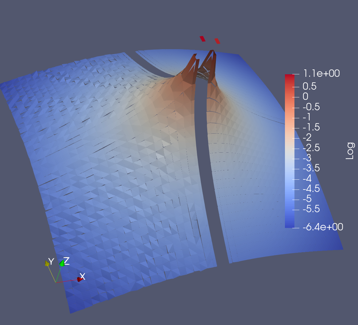
The visualization below shows a logarithmic scale warp of the flux values for both the uncollided algorithm and a LBS simulation using a product quadrature with 96 azimuthal angles and 48 polar angles per octant (18,432 directions total).

The left of the figure is the uncollided algorithm and the right is LBS. Notice the stochastic "noise" from the uncollided algorithm.

The complete program

#include "chi_lua.h"
 
#include "mesh/MeshHandler/chi_meshhandler.h"
#include "mesh/MeshContinuum/chi_meshcontinuum.h"
#include "mesh/Raytrace/raytracing.h"
 
#include "math/SpatialDiscretization/FiniteElement/PiecewiseLinear/pwl.h"
#include "math/RandomNumberGeneration/random_number_generator.h"
#include "math/Quadratures/LegendrePoly/legendrepoly.h"
 
#include "physics/FieldFunction/fieldfunction2.h"
 
#include "chi_runtime.h"
#include "chi_log.h"
 
namespace chi_unit_sim_tests
{
 
int chiSimTest93_RayTracing(lua_State* Lstate)
{
  const std::string fname = "chiSimTest93_RayTracing";
  chi::log.Log() << "chiSimTest93_RayTracing";
 
  //============================================= Get grid
  auto grid_ptr = chi_mesh::GetCurrentHandler().GetGrid();
  const auto& grid = *grid_ptr;
 
  chi::log.Log() << "Global num cells: " << grid.GetGlobalNumberOfCells();
 
  const int dimension = (grid.Attributes() & chi_mesh::DIMENSION_1)? 1 :
                        (grid.Attributes() & chi_mesh::DIMENSION_2)? 2 :
                        (grid.Attributes() & chi_mesh::DIMENSION_3)? 3 : 0;
 
  //============================================= Set parameters
  const size_t num_groups = 1;
  const size_t scattering_order = 1;
  const auto& L = scattering_order;
  const size_t num_moments =
    (dimension == 1)? L + 1 :
    (dimension == 2)? (L+1)*(L+2)/2 :
    (dimension == 3)? (L+1)*(L+1) : 0;
  const double sigma_t = 0.27;
 
  // Build harmonic map
  std::vector<std::pair<int,int>> m_to_ell_em_map;
  if (dimension == 1)
    for (int ell=0; ell<=scattering_order; ell++)
      m_to_ell_em_map.emplace_back(ell,0);
  else if (dimension == 2)
    for (int ell=0; ell<=scattering_order; ell++)
      for (int m=-ell; m<=ell; m+=2)
        m_to_ell_em_map.emplace_back(ell,m);
  else if (dimension == 3)
    for (int ell=0; ell<=scattering_order; ell++)
      for (int m=-ell; m<=ell; m++)
        m_to_ell_em_map.emplace_back(ell,m);
 
  //============================================= Make SDM
  typedef std::shared_ptr<chi_math::SpatialDiscretization> SDMPtr;
  SDMPtr sdm_ptr = chi_math::SpatialDiscretization_PWLD::New(grid_ptr);
  const auto& sdm = *sdm_ptr;
 
  chi_math::UnknownManager phi_uk_man;
  for (size_t m=0; m<num_moments; ++m)
    phi_uk_man.AddUnknown(chi_math::UnknownType::VECTOR_N, num_groups);
 
  const size_t num_fem_local_dofs = sdm.GetNumLocalDOFs(phi_uk_man);
  const size_t num_fem_globl_dofs = sdm.GetNumGlobalDOFs(phi_uk_man);
 
  chi::log.Log() << "Num local FEM DOFs: " << num_fem_local_dofs;
  chi::log.Log() << "Num globl FEM DOFs: " << num_fem_globl_dofs;
 
  //============================================= Define tallies
  std::vector<double> phi_tally(num_fem_local_dofs, 0.0);
 
  //============================================= Define particle
  //                                              data structure
  typedef chi_mesh::Vector3 Vec3;
  struct Particle
  {
    Vec3 position = {0.0,0.0,0.0};
    Vec3 direction = {0.0,0.0,0.0};
    int  energy_group = 0;
    double weight = 1.0;
 
    uint64_t cell_id = 0;
 
    bool alive = true;
  };
 
  //============================================= Define source position
  //                                              and find cell containing it
  const Vec3 source_pos = {0.0,0.0,0.0};
 
  chi_mesh::Cell const* source_cell_ptr = nullptr;
 
  for (auto& cell : grid.local_cells)
    if (grid.CheckPointInsideCell(cell, source_pos))
    {
      source_cell_ptr = &cell;
      break;
    }
  if (source_cell_ptr == nullptr)
    throw std::logic_error(fname + ": Source cell not found.");
 
  const uint64_t source_cell_id = source_cell_ptr->global_id;
 
  //============================================= Define lambdas
  chi_math::RandomNumberGenerator rng;
  auto SampleRandomDirection = [&rng]()
  {
    double costheta = 2.0*rng.Rand() - 1.0;
    double theta    = acos(costheta);
    double varphi   = rng.Rand()*2.0*M_PI;
 
    return chi_mesh::Vector3{sin(theta) * cos(varphi),
                             sin(theta) * sin(varphi),
                             cos(theta)};
  };
 
 
  auto ContributePWLDTally = [&sdm,&grid,&phi_tally,&phi_uk_man,&sigma_t,
                              &num_moments,&m_to_ell_em_map](
    const chi_mesh::Cell& cell,
    const Vec3& positionA,
    const Vec3& positionB,
    const Vec3& omega,
    const int g,
    double weight)
  {
    const auto& cell_mapping = sdm.GetCellMapping(cell);
    const size_t num_nodes = cell_mapping.NumNodes();
 
    const auto phi_theta = chi_math::OmegaToPhiThetaSafe(omega);
    const double phi = phi_theta.first;
    const double theta = phi_theta.second;
 
    std::vector<double> segment_lengths;
    chi_mesh::PopulateRaySegmentLengths(grid,             //input
                                        cell,             //input
                                        positionA,        //input
                                        positionB,        //input
                                        omega,            //input
                                        segment_lengths); //output
 
    std::vector<double> shape_values_k;   //At s_k
    std::vector<double> shape_values_kp1; //At s_{k+1}
 
    cell_mapping.ShapeValues(positionA,       //input
                             shape_values_k); //output
 
    double d_run_sum = 0.0;
    for (const auto& segment_length_k : segment_lengths)
    {
      d_run_sum += segment_length_k;
      const double& d = d_run_sum;
 
      cell_mapping.ShapeValues(positionA+omega*d, shape_values_kp1);
 
      const auto&   b_ik   = shape_values_k;
      const auto&   b_ikp1 = shape_values_kp1;
      const double& ell_k  = segment_length_k;
 
      for (size_t i=0; i<num_nodes; ++i)
      {
        const double C0 = b_ik[i] * ell_k;
        const double C1 = b_ikp1[i] - b_ik[i];
 
        for (size_t m=0; m < num_moments; ++m)
        {
          const int64_t dof_map = sdm.MapDOFLocal(cell, i, phi_uk_man, m, g);
 
          //================= Apply harmonic weight
          const auto& ell_em = m_to_ell_em_map.at(m);
          const int ell = ell_em.first;
          const int em = ell_em.second;
 
          double w_harmonic = chi_math::Ylm(ell, em, phi, theta);
 
          //================= Apply exponential attenuation weight
          double w_exp  = (C0 / sigma_t) * (1.0 - exp(-sigma_t * ell_k)) +
                          (C1 / (sigma_t * sigma_t)) *
                          (1.0 - (1 + sigma_t * ell_k) * exp(-sigma_t * ell_k));
                 w_exp *= weight / (ell_k * ell_k);
 
          //================= Combine
          double w_avg = w_harmonic * w_exp;
 
          phi_tally[dof_map] += ell_k * w_avg ;
        }//for moment m
      }//for node i
 
      shape_values_k = shape_values_kp1;
      weight *= exp(-sigma_t * segment_length_k);
    }//for d
  };
 
  auto GetCellApproximateSize = [&grid](const chi_mesh::Cell& cell)
  {
    const auto& v0 = grid.vertices[cell.vertex_ids[0]];
    double xmin = v0.x, xmax = v0.x;
    double ymin = v0.y, ymax = v0.y;
    double zmin = v0.z, zmax = v0.z;
 
    for (uint64_t vid : cell.vertex_ids)
    {
      const auto& v = grid.vertices[vid];
 
      xmin = std::min(xmin, v.x); xmax = std::max(xmax, v.x);
      ymin = std::min(ymin, v.y); ymax = std::max(ymax, v.y);
      zmin = std::min(zmin, v.z); zmax = std::max(zmax, v.z);
    }
 
    return (chi_mesh::Vector3(xmin, ymin, zmin) -
            chi_mesh::Vector3(xmax, ymax, zmax)).Norm();
  };
 
  //============================================= Create raytracer
  std::vector<double> cell_sizes(grid.local_cells.size(), 0.0);
  for (const auto& cell : grid.local_cells)
    cell_sizes[cell.local_id] = GetCellApproximateSize(cell);
 
  chi_mesh::RayTracer ray_tracer(grid, cell_sizes);
 
  //============================================= Run rays
  const size_t num_particles = 1'000'000;
  for (size_t n=0; n<num_particles; ++n)
  {
    if (n % size_t(num_particles/10.0) == 0)
      std::cout << "#particles = " << n << "\n";
    //====================================== Create the particle
    const auto omega = SampleRandomDirection();
    Particle particle{source_pos,     //position
                      omega,          //direction
                      0,              //e_group
                      1.0,            //weight
                      source_cell_id, //cell_id
                      true};          //alive
 
    while (particle.alive)
    {
      //=============================== Get the current cell
      const auto& cell = grid.cells[particle.cell_id];
 
      //=============================== Perform the trace
      //                                to the next surface
      auto destination_info = ray_tracer.TraceRay(cell,
                                                  particle.position,
                                                  particle.direction);
 
      const Vec3& end_of_track_position = destination_info.pos_f;
 
      //=============================== Make tally contribution
      ContributePWLDTally(cell,
                          particle.position,     //positionA
                          end_of_track_position, //positionB
                          particle.direction,    //omega
                          particle.energy_group, //g
                          particle.weight);      //weight at A
 
      //=============================== Process cell transfer
      //                                or death
      if (not destination_info.particle_lost)
      {
        const auto& f = destination_info.destination_face_index;
        const auto& current_cell_face = cell.faces[f];
 
        if (current_cell_face.has_neighbor)
          particle.cell_id = current_cell_face.neighbor_id;
        else
          particle.alive = false; //Death at the boundary
      }
      else
      {
        std::cout << "particle" << n << " lost "
                  << particle.position.PrintStr() << " "
                  << particle.direction.PrintStr() << " "
                  << "\n";
        break;
      }
 
      const auto& pA = particle.position;
      const auto& pB = end_of_track_position;
      particle.weight *= exp(-sigma_t*(pB-pA).Norm()); //Attenuation
      particle.position = end_of_track_position;
    }//while ray alive
 
  }//for ray n
 
  //============================================= Post process tallies
  for (const auto& cell : grid.local_cells)
  {
    //====================================== Compute mass matrix
    //                                       and its inverse
    const auto& cell_mapping = sdm.GetCellMapping(cell);
    const auto& qp_data = cell_mapping.MakeVolumeQuadraturePointData();
    const size_t num_nodes = cell_mapping.NumNodes();
 
    MatDbl M(num_nodes, VecDbl(num_nodes, 0.0));
    for (auto qp : qp_data.QuadraturePointIndices())
      for (size_t i=0; i<num_nodes; ++i)
        for (size_t j=0; j<num_nodes; ++j)
          M[i][j] += qp_data.ShapeValue(i,qp) * qp_data.ShapeValue(j, qp) *
                     qp_data.JxW(qp);
 
    auto M_inv = chi_math::Inverse(M);
 
    //====================================== Apply projection
    VecDbl T(num_nodes, 0.0);
    for (size_t m=0; m<num_moments; ++m)
      for (size_t g=0; g<num_groups; ++g)
      {
        for (size_t i=0; i<num_nodes; ++i)
        {
          const int64_t imap = sdm.MapDOFLocal(cell, i, phi_uk_man, m, g);
          T[i] = phi_tally[imap] / num_particles;
        }
 
        auto phi_uc = chi_math::MatMul(M_inv, T);
 
        for (size_t i=0; i<num_nodes; ++i)
        {
          const int64_t imap = sdm.MapDOFLocal(cell, i, phi_uk_man, m, g);
          phi_tally[imap] = phi_uc[i];
        }
      }//for group g
 
  }//for cell
 
  //============================================= Create Field Functions
  std::vector<std::shared_ptr<chi_physics::FieldFunction>> ff_list;
 
  ff_list.push_back(std::make_shared<chi_physics::FieldFunction>(
    "Phi",                                           //Text name
    sdm_ptr,                                         //Spatial Discr.
    chi_math::Unknown(chi_math::UnknownType::VECTOR_N,num_groups) //Unknown
  ));
 
  //============================================= Localize zeroth moment
  //This routine extracts a single moment vector
  //from the vector that contains multiple moments
  const chi_math::UnknownManager m0_uk_man(
    {chi_math::Unknown(chi_math::UnknownType::VECTOR_N,num_groups)});
  const size_t num_m0_dofs = sdm.GetNumLocalDOFs(m0_uk_man);
 
  std::vector<double> m0_phi(num_m0_dofs, 0.0);
 
  sdm.CopyVectorWithUnknownScope(phi_tally,     //from vector
                                 m0_phi,      //to vector
                                 phi_uk_man,  //from dof-structure
                                 0,           //from unknown-id
                                 m0_uk_man,   //to dof-structure
                                 0);          //to unknown-id
 
  ff_list[0]->UpdateFieldVector(m0_phi);
 
 
  //============================================= Update field function
  chi_physics::FieldFunction::FFList const_ff_list;
  for (const auto& ff_ptr : ff_list)
    const_ff_list.push_back(ff_ptr);
  chi_physics::FieldFunction::ExportMultipleToVTK(fname,
                                                   const_ff_list);
 
  return 0;
}
 
}//namespace chi_unit_sim_tests

Table of Contents